Anomaly detection using Isolation Forest and Local Outlier Factor

“Alert if CPU rises above 95%, but only if it stays there for three polling cycles.”

Anomalies are data points in a dataset that are different from the normal state of existence and contradict the data’s expected behavior. Anomalies in data are also called standard deviations, outliers, noise, novelties, and exceptions.

There are three types of anomalies:

Point anomalies: It is when a single instance of data is anomalous.

Contextual anomalies: It is when the abnormality is context-specific. It is common in time-series data.

Collective anomalies: It is when a set of data instances collectively helps in detecting anomalies.

In machine learning and data mining, anomaly detection is the task of identifying the rare items, events or observations which are suspicious and seem different from the majority of the data. These anomalies can indicate some kind of problems such as bank fraud, medical problems, failure of industrial equipment, etc.

The anomaly detection methods are categorized into supervised and unsupervised machine learning approaches.

Supervised anomaly detection techniques require a data set with a complete set of “normal” and “abnormal” labels in order for a classification algorithm to work.

Unsupervised anomaly detection methods detect anomalies in an unlabeled test set of data solely based on the data’s intrinsic properties.

A few popular techniques used for anomaly detection are listed below:-

1. Isolation Forest
2. Local Outlier Factor
3. K-Nearest Neighbor's
4. One-Class Support Vector Machine
5. Neural Networks and Autoencoders

This article focuses on first two techniques, which are isolation forest and local outlier factor and understand these techniques in brief with hands-on implementation of these techniques.

Isolation Forest:

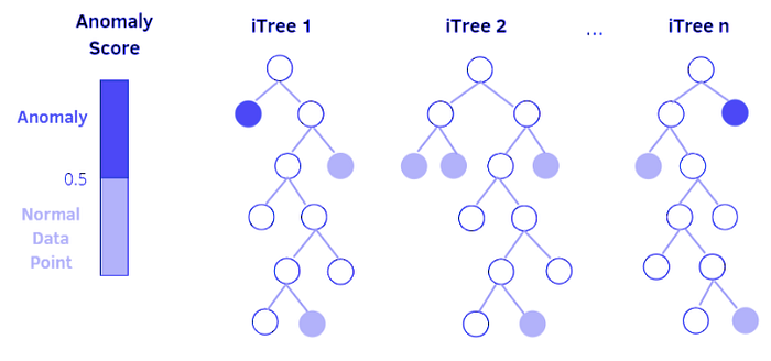
The isolation forest algorithm detects anomalies using a tree-based approach. It is based on modelling normal data in order to isolate anomalies that are both few in number and distinct in the feature space. The algorithm essentially accomplishes this by generating a random forest in which decision trees are grown at random; at each node, features are chosen at random, and a random threshold value is chosen to divide the dataset in half.

It keeps cutting away at the dataset until all instances are isolated from one another. Because an anomaly is usually far away from other instances, it becomes isolated in fewer steps than normal instances on average (across all decision trees).

Local Outlier Factor:

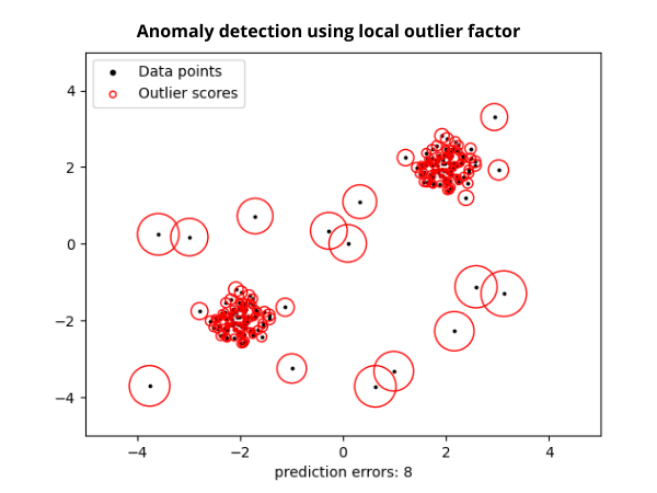
A local outlier factor is an algorithm that is used to find anomalous data points by measuring the local deviation of a given data point with respect to its neighbors.

The local outlier factor algorithm considers the distances of K-nearest neighbor's from a core point to estimate the density. By comparing the local density of an object to the local densities of its neighbor’s, the regions of similar density and points that have a substantially lower density than their neighbor's can be identified. These points are considered outliers by the algorithm. This is how the anomalies are detected by using this algorithm.

Hands-on Implementation:

Let’s apply above two anomaly detection algorithms to real-world datasets. The dataset considered here contains information on 25 different features of Credit card payment defaults.

To read this data we are using the Pandas library. Let’s first load the data and visualize the top 5 rows of it.

# Import pandas
import pandas as pd

# Load the data
data = pd.read_csv('https://raw.githubusercontent.com/analyticsindiamagazine/MocksDatasets/main/Credit_Card.csv')

# Top 5 rows
data.head()

Let’s check the shape of the dataset

# Check the shape
Data.shape

Now before moving to the modelling let’s first check the distribution of one of the input features using famous data visualization libraries like Matplotlib

# import matplotlib
import matplotlib.pyplot as plt
# See how data is spreaded
plt.figure(figsize=(8,6))
plt.hist(X[:,4])
plt.xlabel('Age')
plt.ylabel('Frequency of datapoints')

Step 3: Initialize and train the IF and LOF

Let’s import the Isolation forest and Local outlier factor from the sklearn library and will train those on our training pattern

# Import IF and LOF
from sklearn.ensemble import IsolationForest
from sklearn.neighbors import LocalOutlierFactor
# Initialize and train the IF
IF = IsolationForest(random_state=0)
IF.fit(X)

# Initialize and train LOF
LOF = LocalOutlierFactor()
LOF.fit(X)

Step 4: Predicting and plotting anomalies:

We have successfully trained both algorithms, here we will now obtain the prediction from each algorithm and will plot anomalies.

# Anomalies given by IF
IF_anomalies = IF.predict(X)
  
# Plotting anomalies given by IF
plt.figure(figsize=(8,6))
plt.hist(X[:,4],label='Normal')
plt.hist(X[IF_anomalies==-1][:,4], color='red', label='Anomalies')
plt.xlabel('Age of the customers')
plt.ylabel('Frequency')
plt.ylim((0,6000))
plt.legend()

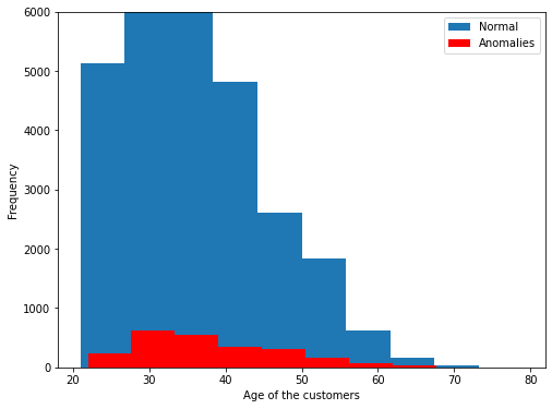
The distribution in red color represents anomalies, we can read it as around 2300 customers from age 21 to 67 are something which is insignificant or abnormal.

Now let’s plot anomalies identified by the LOF.

# Anomalies given by the LOF
LOF_anomalies = LOF.fit_predict(X)
# Plotting anomalies given by LOF
plt.figure(figsize=(8,6))
plt.hist(X[:,4],label='Normal')
plt.hist(X[LOF_anomalies==-1][:,4], color='red', label='Anomalies')
plt.xlabel('Age of the customers')
plt.ylabel('Frequency')
plt.ylim((0,6000))
plt.legend()

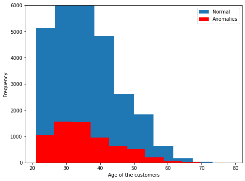
The anomalies identified by the LOF are between the ages of 21 to 69 and those are around 6544. From the above two outputs, it looks like the LOF is giving more information on anomalies. The quality of both results can be well assed by the domain expert.

So this is how we can use Isolation forest and Local outlier factors to detect anomalies in the real-world datasets.